Validating the costDist migration • traveltime

calculate_travel_time() used to convert the terra friction surface to a raster object so it could run the gdistance cost-distance pipeline. That pulled in two dependencies — raster (superseded by terra) and gdistance — purely as machinery. The function has since been reimplemented on terra::costDist() and those dependencies dropped.

This article is the evidence that the switch was safe: that terra::costDist() reproduces the same calculation. Both approaches use the same cost model — eight-direction movement between cell centres, with each step costing distance * mean(friction) of the two cells. The claim to defend is that the two differ only by:

the geodesic distance used (terra computes true geodesic inter-cell distances; gdistance::geoCorrection() used an approximation), and
a half-cell convention at the origins (gdistance charges half of the origin cell’s own friction on the first step; costDist() measures cost to the border of the origin cell and omits it),

and by nothing else. Written as a decomposition:

$\underbrace{\text{costDist} - \text{gdistance}}_{\text{raw difference}} \;=\; \underbrace{\text{geodesic effect}}_{\text{true} - \text{approx distance}} \;+\; \underbrace{\text{origin half-cell}}_{\approx\,\tfrac{1}{2}\text{ cell of friction}} \;+\; \underbrace{0}_{\text{everything else}}$

The last term is the one worth proving. The two experiments below drive it to zero.

library(traveltime)
library(terra)
library(gdistance)
library(raster)

The original pipeline, kept here only for comparison:

# gdistance builds a graph with edge cost distance * mean(friction) and
# accumulates least-cost paths -- exactly the model terra::costDist() uses.
tt_gdistance <- function(fs, points) {
  fr  <- raster::raster(fs)
  tgc <- gdistance::geoCorrection(
    gdistance::transition(fr, function(x) 1 / mean(x), 8)
  )
  tt <- gdistance::accCost(tgc, as.matrix(points[, 1:2]))
  names(tt) <- "travel_time"
  out <- terra::rast(tt)
  terra::crs(out) <- terra::crs(fs)   # align CRS string for raster arithmetic
  out
}

The trick that isolates the two effects: re-run gdistance with the origin cells’ friction set to ~0. That removes the half-cell term, so any remaining difference against costDist() is the geodesic term alone.

1. In a projected CRS the two maps are identical to machine precision

A projected coordinate system makes the geodesic term exactly zero by construction — all inter-cell distances are planar and both methods use the same ones. So the only thing that can differ is the origin convention. Once we remove that, every cell must agree.

utm  <- "+proj=utm +zone=32 +datum=WGS84"
frP  <- make_friction(180, 180, 0, 18000, 0, 18000, utm, seed = 3)
ptsP <- data.frame(x = c(3200, 13800), y = c(4200, 12800))

new  <- calculate_travel_time(frP, ptsP)          # terra::costDist
old  <- tt_gdistance(frP, ptsP)                   # gdistance

# neutralise the origin cells' friction to remove the half-cell term
cn   <- terra::cellFromXY(frP, as.matrix(ptsP[, 1:2]))
fs0  <- frP; fs0[cn] <- 1e-9
old0 <- tt_gdistance(fs0, ptsP)                   # gdistance, no half-cell

x  <- terra::values(new)[, 1]
y  <- terra::values(old)[, 1]
y0 <- terra::values(old0)[, 1]
ok <- is.finite(x) & is.finite(y) & is.finite(y0)

d_raw   <- new - old        # raw difference
d_resid <- new - old0       # residual after removing the origin half-cell
offset  <- median((y - x)[ok])                     # the half-cell offset
resid_max <- max(abs(terra::values(d_resid)), na.rm = TRUE)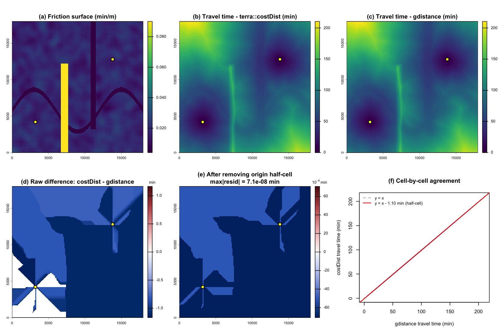

Projected CRS. (a) friction surface with two low-friction corridors and a high-friction barrier; origins in yellow. (b, c) travel time from costDist and gdistance – visually identical. (d) raw difference: a near-constant offset localised to the origins. (e) after removing the origin half-cell, the residual is flat at the 1e-9 min level across the whole map. (f) every cell lies on a single line offset from y = x by exactly the half-cell.

The travel-time maps (b, c) are indistinguishable: the same barrier shadow, the same corridor short-cuts. The raw difference (d) is a near-constant offset of about 1.1 min, with structure only in the immediate neighbourhood of the origins — that is the half-cell. Remove it and the residual (e) is flat at the 7e-08 min level across all 32,400 cells; the faint texture there is floating-point noise, not signal. Panel (f) says the same thing: every cell sits on one line parallel to y = x, offset by exactly the half-cell.

In a projected CRS, then, the two calculations are the same to machine precision once the origin convention is accounted for — the cost model, the neighbourhood, and the accumulation all carry over exactly.

2. At high latitude, the only remainder is a small geodesic field

Now repeat on a longitude/latitude surface at 55°N, where meridians converge and the geodesic term is live. After removing the same origin half-cell, whatever is left is the pure geodesic effect.

frG  <- make_friction(150, 150, 10, 11, 55, 56, "EPSG:4326", seed = 7,
                      lo = 0.015, hi = 0.04)
ptsG <- data.frame(x = c(10.25, 10.78), y = c(55.22, 55.75))

newG  <- calculate_travel_time(frG, ptsG)
oldG  <- tt_gdistance(frG, ptsG)
cnG   <- terra::cellFromXY(frG, as.matrix(ptsG[, 1:2]))
fs0G  <- frG; fs0G[cnG] <- 1e-9
old0G <- tt_gdistance(fs0G, ptsG)

xg <- terra::values(newG)[, 1]
yg <- terra::values(oldG)[, 1]
y0g <- terra::values(old0G)[, 1]
okg <- is.finite(xg) & is.finite(yg) & is.finite(y0g)

d_raw_G   <- newG - oldG
d_resid_G <- newG - old0G                 # geodesic effect only
rg        <- terra::values(d_resid_G)[, 1]

# relative size, on well-resolved cells only (at the origins travel time -> 0,
# so a per-cell ratio there is a meaningless 0/0)
tt_thr  <- 0.05 * max(yg[okg])
sel     <- okg & yg > tt_thr
relf    <- 100 * abs(rg[sel]) / yg[sel]
med_rel <- median(relf)
p95_rel <- quantile(relf, 0.95)
resid_max_G <- max(abs(rg), na.rm = TRUE)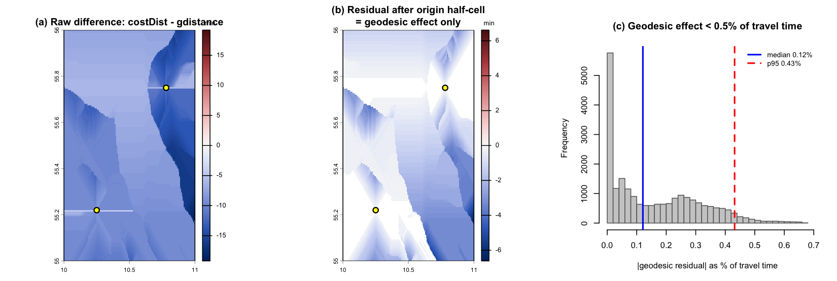

Lon/lat at 55N. (a) raw difference. (b) residual after removing the origin half-cell – a smooth geodesic field with no local structure. (c) that residual as a percentage of travel time on well-resolved cells: under half a percent.

The residual (b) is not noise and not local: it is a smooth, large-scale field, exactly the signature of a distance-model difference rather than a bug. As a fraction of travel time (c) it is tiny — median 0.12%, 95th percentile 0.43%, peaking at 6.6 min over travel times of hundreds of minutes. And here terra is the more accurate of the two: it uses true geodesic inter-cell distances, where gdistance::geoCorrection() only approximated them.

Conclusion

Barring the geodesic distance model and the half-cell origin convention, the two methods are the same calculation — and in the projected case, where the geodesic term vanishes, that sameness is exact to floating-point precision at every cell. That is what justified dropping raster and gdistance: the cost model, the neighbourhood, and the accumulation all carry over to terra::costDist() unchanged, with the geographic correction now performed internally and more accurately.

The same comparison is run numerically (including on the real Singapore walk2020 surface) in data-raw/compare_costdist_vs_gdistance.R, data-raw/singapore_compare.R, and data-raw/compare_costdist_plots.R, with results summarised in data-raw/costdist_migration_comparison.md.