Calculate Travel Times Over Space • traveltime

traveltime enables a user to create a map of travel time over an area of interest from a user-specified set of geographic coordinates and friction surface. The package provides convenient access to global friction surfaces for walking and motorised travel for the year 2020. The final result is a raster of the area of interest where the value in each cell is the lowest travel time in minutes to any of the specified locations.

Walking travel time from rail transport in Singapore

Installation

install.packages("traveltime", repos = c("https://idem-lab.r-universe.dev"))

remotes::install_github("idem-lab/traveltime")

Documentation

Website

https://idem-lab.github.io/traveltime/

Paper

Ryan, G.E., Tierney, N., Golding, N., and Weiss, D.J (2025). traveltime: an R package to calculate travel time across a landscape from user-specified locations. EarthArXiv 10.31223/X56M74

What does this thing do?

The traveltime workflow starts with:

a set of points you are interested in,

and either

you supply a friction surface for the area you are interested in, or
you supply your area of interest and use get_friction_surface to retrieve a pre-prepared walking or motorised travel friction surface from Weiss et al. (2020) ¹ — this will probably be the case in most applications.

Then, running calculate_travel_time produces a raster as a terra SpatRaster with the travel time to the (temporally) nearest of the supplied points over the area of interest.

A practical example: walking from public transport in Singapore

Here we will calculate the walking travel time from the nearest mass transit station across the island nation of Singapore — specifically Mass Rapid Transit (MRT) and Light Rail Transit (LRT) stations — and create a map of this.

Prepare the data

For this exercise, we need two items of data:

our points to calculate travel time from — here the locations of Singapore’s MRT and LRT stations, and
our area of interest — in this case a map of Singapore.

Points

Our points of interest will be the stations data set included in traveltime; a 563 row, 2 column matrix containing the longitude (x) and latitude (y) of all LRT and MRT station exits in Singapore from ²:

library(traveltime)
head(stations)
#>             x        y
#> [1,] 103.9091 1.334922
#> [2,] 103.9335 1.336555
#> [3,] 103.8493 1.297699
#> [4,] 103.8508 1.299195
#> [5,] 103.9094 1.335311
#> [6,] 103.9389 1.344999

Area of interest

To obtain our area of interest, we download a national-level polygon boundary of Singapore using the geodata package. Here we download only the national boundary (level = 0) at a low resolution (resolution = 2). Our boundary singapore_shapefile is a SpatVector class object from the package terra.

library(terra)
#> terra 1.8.5
library(geodata)

singapore_shapefile <- gadm(
  country = "Singapore",
  level = 0,
  path = tempdir(),
  resolution = 2
)

singapore_shapefile
#>  class       : SpatVector 
#>  geometry    : polygons 
#>  dimensions  : 1, 2  (geometries, attributes)
#>  extent      : 103.6091, 104.0858, 1.1664, 1.4714  (xmin, xmax, ymin, ymax)
#>  coord. ref. : lon/lat WGS 84 (EPSG:4326) 
#>  names       : GID_0   COUNTRY
#>  type        : <chr>     <chr>
#>  values      :   SGP Singapore

Friction surface

Now that we have the two items of data that we require initially, the next step is to prepare a friction surface for our area of interest.

We will use the friction surface from Weiss et al. (2020) that can be downloaded by traveltime with the function get_friction_surface(). This function takes extents in a variety of formats and returns the surface for that extent only.

We can pass in our basemap singapore_shapefile, a SpatVector, directly as the extent. We’re interested in walking time from a station, so we’ll download the walking friction surface by specifying surface = "walk2020".

(Alternatively, we could use surface = "motor2020" for motorised travel).

We’re only interested in walking on land, so we then mask out areas outside of the land boundary of singapore_shapefile:

friction_singapore <- get_friction_surface(
    surface = "walk2020",
    extent = singapore_shapefile
  )|> 
  mask(singapore_shapefile)
#> Checking if the following Surface-Year combinations are available to download:
#> 
#>     DATASET ID  YEAR
#>   - Accessibility__202001_Global_Walking_Only_Friction_Surface:  DEFAULT
#> 
#> Loading required package: sf
#> Linking to GEOS 3.13.0, GDAL 3.10.0, PROJ 9.5.1; sf_use_s2() is FALSE
#> No encoding supplied: defaulting to UTF-8.
#> <GMLEnvelope>
#> ....|-- lowerCorner: 1.1664 103.6091
#> ....|-- upperCorner: 1.4714 104.0858Start tag expected, '<' not found

Thus we have our friction surface as a SpatRaster:

friction_singapore
#> class       : SpatRaster 
#> dimensions  : 37, 57, 1  (nrow, ncol, nlyr)
#> resolution  : 0.008333333, 0.008333333  (x, y)
#> extent      : 103.6083, 104.0833, 1.166667, 1.475  (xmin, xmax, ymin, ymax)
#> coord. ref. : lon/lat WGS 84 (EPSG:4326) 
#> source(s)   : memory
#> varname     : Accessibility__202001_Global_Walking_Only_Friction_Surface_1.1664,103.6091,1.4714,104.0858 
#> name        : friction_surface 
#> min value   :       0.01200000 
#> max value   :       0.06192715

Input data

Below we plot the friction surface raster friction_singapore, with the vector boundary singapore_shapefile as a grey line, and stations as grey points. traveltime takes resistance values of friction (see paper for more details), so higher values of friction indicate more time travelling across a given cell.

library(tidyterra)
#> Registered S3 method overwritten by 'tidyterra':
#>   method              from        
#>   autoplot.SpatRaster malariaAtlas
#> 
#> Attaching package: 'tidyterra'
#> The following object is masked from 'package:stats':
#> 
#>     filter
library(ggplot2)

ggplot() +
  geom_spatraster(
    data = friction_singapore
  ) +
  geom_spatvector(
    data = singapore_shapefile,
    fill = "transparent",
    col = "grey50"
  ) +
  geom_point(
    data = stations,
    aes(
      x = x,
      y = y
    ),
    col = "grey60",
    size = 0.5
  ) +
  scale_fill_viridis_c(
    option = "A",
    na.value = "transparent",
    direction = -1
  ) +
  labs(
    fill = "Resistance",
    x = element_blank(),
    y = element_blank()
  ) +
  theme_minimal()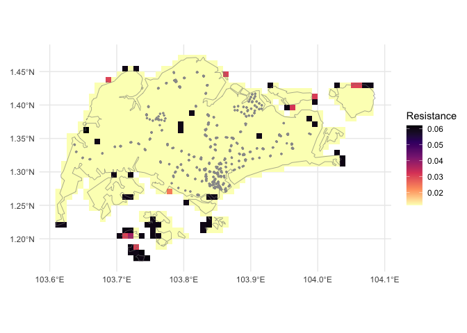

Friction surface raster of Singapore, showing Singapore boundary in grey, and station locations as grey points.

Calculate travel time

With all the data collected, the function calculate_travel_time() takes the friction surface friction_singapore and the points of interest in stations, and returns a SpatRaster of walking time in minutes to each cell from the nearest station:

trave_time_singapore <- calculate_travel_time(
  friction_surface = friction_singapore,
  points = stations
)

trave_time_singapore
#> class       : SpatRaster 
#> dimensions  : 37, 57, 1  (nrow, ncol, nlyr)
#> resolution  : 0.008333333, 0.008333333  (x, y)
#> extent      : 103.6083, 104.0833, 1.166667, 1.475  (xmin, xmax, ymin, ymax)
#> coord. ref. :  
#> source(s)   : memory
#> name        : travel_time 
#> min value   :           0 
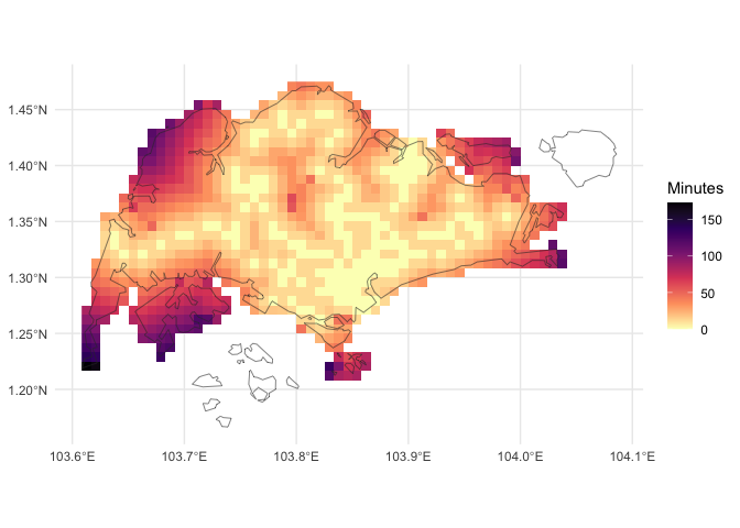
#> max value   :         Inf

Plot results

We present the resulting calculated travel times below where (as expected) the travel times are lowest near station exits and progressively higher further away. Note that the results in trave_time_singapore include infinite values (Inf above). The islands to the south and north-east are shown as filled cells in the figure above, i.e., they are not masked out by singapore_shapefile. But because those islands they are not connected to any cells with a station, the calculated travel time is infinite, and so these cells do not appear in the figure below.

ggplot() +
  geom_spatraster(
    data = trave_time_singapore
  ) +
  scale_fill_viridis_c(
    option = "A",
    direction = -1,
    na.value = "transparent"
  ) +
  theme_minimal() +
  labs(fill = "Minutes") +
  geom_spatvector(
    data = singapore_shapefile,
    fill = "transparent",
    col = "grey20"
  )

Map of walking travel time in Singapore, in minutes from nearest MRT or LRT station.